The Astrophysical Journal, 543:178-194, 2000 November 1
© 2000. The American Astronomical Society. All rights reserved. Printed in U.S.A.
Nearby Optical Galaxies: Selection of the Sample and Identification of Groups
Giuliano Giuricin ,1,2 Christian Marinoni ,1 Lorenzo Ceriani ,1 and Armando Pisani 3
Received 1999 July 26; accepted 2000 June 5
ABSTRACT
In this paper we describe the Nearby Optical Galaxy (NOG) sample, which is a complete, distance-limited (cz  6000 km s-1) and magnitude-limited (B 14) sample of
  7000 optical galaxies. The sample covers
 (8.27 sr) of the sky (|b| > 20
 ) and appears to have a good completeness in redshift (97%). We select the sample on the basis of homogenized corrected total blue magnitudes in order to minimize systematic effects in galaxy sampling. We identify the groups in this sample by means of both the hierarchical and the percolation "friends-of-friends" methods. The resulting catalogs of loose groups appear to be similar and are among the largest catalogs of groups currently available. Most of the NOG galaxies (60%) are found to be members of galaxy pairs (580 pairs for a total of 15% of objects) or groups with at least three members (500 groups for a total of 45% of objects). About 40% of galaxies are left ungrouped (field galaxies). We illustrate the main features of the NOG galaxy distribution. Compared to previous optical and IRAS galaxy samples, the NOG provides a denser sampling of the galaxy distribution in the nearby universe. Given its large sky coverage, the identification of groups, and its high-density sampling, the NOG is suited to the analysis of the galaxy density field of the nearby universe, especially on small scales.
Subject headings: galaxies: clusters: general galaxies: distances and redshiftslarge-scale structure of universe
1 Dipartimento di Astronomia, Universitŕ degli Studi di Trieste, via G. B. Tiepolo 11, Trieste 34131, Italy; giuricin@sissa.it, marinoni@sissa.it, ceriani@sissa.it.
2 SISSA, via Beirut 4, 34013, Trieste, Italy.
3 Osservatorio Astronomico, via G. B. Tiepolo 11, Trieste 34131, Italy; pisani@ts.astro.it.
1. INTRODUCTION
With the advent of large surveys of galaxy redshifts coupled to well-selected galaxy catalogs, it has become possible to delineate the three-dimensional distribution of galaxies and to attempt a three-dimensional definition of the galaxy density.
This paper, which is the third in a series of papers (Marinoni et al. 1998, 1999, hereafter Papers I and II, respectively) in which we investigate the properties of the large-scale galaxy distribution, presents the all-sky sample of optical galaxies used in our study and the identification of galaxy groups in this sample.
The first three-dimensional galaxy catalog that covered both Galactic hemispheres with good completeness in redshift was the magnitude-limited (B  12 mag) Revised Shapley-Ames Catalog of Bright Galaxies (RSA; Sandage & Tammann 1981). It was used by Yahil, Sandage, & Tammann (1980) to calculate the galaxy density field in the Local Supercluster (LS). The structures of the LS region were well delineated by Tully & Fisher (1987) on the basis of the Nearby Galaxies Catalog (NBG; Tully 1988), which is a combination of the RSA catalog and a diameter-limited sample of late-type and fainter galaxies found in an all-sky H I survey. This catalog, which is limited to a depth of 3000 km s-1 and is complete down to B 12 mag (although it extends to fainter magnitudes), was also used to determine local galaxy density parameters, which were exploited in statistical analyses of environmental effects on some properties of the LS galaxies (Giuricin et al. 1993, 1994, 1995; Monaco et al. 1994).
In an effort to go beyond the LS, Hudson (1993a, 1993b, 1994a, 1994b) constructed a wide galaxy sample from a merging of the diameter-limited northern Uppsala General Catalogue of Galaxies (UGC; Nilson 1973) and the diameter-limited southern ESO catalog (Lauberts 1982; Lauberts & Valentijn 1989). He applied statistical corrections for the fairly large incompleteness in redshift of his sample as a function of angular diameter and position on the sky and reconstructed the density field of optical galaxies to a depth of cz = 8000 km s-1.
The Optical Redshift Survey (ORS; Santiago et al. 1995), which provided 1300 new redshifts for bright and nearby galaxies, marks a considerable advance toward the construction of an all-sky sample of nearby optical galaxies with good completeness in redshift. The ORS contains 8300 galaxies with known redshift and consists of two overlapping optically selected samples (limited in apparent magnitude and diameter, respectively), which cover almost all the sky with |b| > 20. Each sample is the concatenation of three subsamples drawn from the UGC catalog in the north, the ESO catalog in the south (for  < -17
< -17 5), and the extension to the Southern Galaxies Catalogue (ESGC; H. G. Corwin & B. A. Skiff 1999 in preparation) in the strip between the UGC and ESO regions (-175 -25). The authors selected their own galaxy sample according to the raw (observed) magnitudes and diameters and then attempted to quantify the effects of Galactic extinction on the galaxy density field as well as the effects of random errors and systematic trends in the magnitude and diameter scales internal to different catalogs. They calculated the galaxy density field out to cz = 8000 km s-1 in redshift space on the basis of the UGC and ESO magnitude-limited samples and of the ESGC diameter-limited sample (for a total of 6400 galaxies), after having collapsed the galaxy members of six rich nearby clusters to a single redshift (Santiago et al. 1996). Baker et al. (1998) calculated the peculiar-velocity field resulting from the ORS sample (defined as above), adding the IRAS 1.2 Jy galaxy sample (Fisher et al. 1995) in the unsurveyed zone of avoidance (ZOA; |b| < 20) and at large distances (cz > 8000 km s-1).
In this paper, we follow a different approach to the construction of an all-sky sample of optical galaxies with good properties of completeness, by attempting to use a uniform selection criterion (based on homogenized blue magnitudes corrected for Galactic extinction, internal extinction, and K dimming) over the sky. The sample we select (hereafter the Nearby Optical Galaxy [NOG] sample) is a complete, magnitude- and distance-limited, all-sky sample of 7000 nearby and bright optical galaxies, which we extract from the Lyon-Meudon Extragalactic Database (LEDA; e.g., Paturel et al. 1997).
This sample constitutes an extension in distance and in the number of redshifts (with a consequent increase in redshift completeness) of the all-sky sample of 6400 bright and nearby galaxies (5400 galaxies above |b| = 20), recently used in the calculation of different sets of galaxy distances corrected for noncosmological motions by means of peculiar-velocity field models (Paper I) and in the rediscussion of the local galaxy luminosity function (Paper II).
As previously emphasized (e.g., Hudson 1993a; Santiago et al. 1995), outside the ZOA, optical galaxy samples are more suitable for mapping the galaxy density field on small scales than IRAS-selected galaxy samples, which have been frequently used as tracers of the galaxy density field on large scales (e.g., Strauss et al. 1992, based on the IRAS 1.9 Jy sample; Fisher et al. 1995 and Webster, Lahav, & Fisher 1997, both based on the IRAS 1.2 Jy sample; Branchini et al. 1999 and Schmoldt et al. 1999, both based on the Point-Source Catalog Redshift [PSCz] sample by Saunders et al. 2000a, 2000b), because IRAS samples do not include the early-type galaxies (which have little dust content and star formation), are relatively sparse nearby, and are based on far-infrared fluxes, which are much less linked with galaxy mass than optical and near-infrared fluxes. The latter are believed to be the best tracers of galaxy mass, and this motivates ongoing plans for constructing wide magnitude-limited samples of near-infrared selected galaxies, such as the 2MASS (e.g., Huchra et al. 2000) and DENIS (e.g., Epchtein et al. 1999) projects.
Moreover, as discussed by Santiago et al. (1996), standard extinction corrections on diameters are thought to be less reliable than extinction corrections on magnitudes. This makes it preferable to use magnitude-limited optical samples rather than diameter-limited optical ones for the reconstruction of the galaxy density field.
Since we plan to use the NOG sample to trace the galaxy density field on small scales as well, in this paper we provide group assignments for the galaxies of the NOG sample by means of both the hierarchical (H; e.g., Tully 1987) and the percolation (P) friends-of-friends methods (e.g., Huchra & Geller 1982) of group identification. The identification of groups, which allow us to study the continuity of the properties of galaxy systems over a large range of scales (e.g., Girardi & Giuricin 2000), is also useful for improving the determination of the three-dimensional structure (e.g., the groups identified by Wegner, Haynes, & Giovanelli 1993 in the Perseus-Pisces region). Furthermore, galaxy systems are favorite targets for determining the peculiar-velocity field with reduced uncertainties (e.g., Giovanelli et al. 1997). In a forthcoming paper we will use the locations of individual galaxies and groups to reconstruct the galaxy density field (see Marinoni et al. 2000 for preliminary results).
The outline of our paper is as follows. In § 2 we present the selection of the NOG sample. In § 3 we illustrate the distribution of NOG galaxies on the sky. In § 4 we summarize the two identification procedures of groups, i.e., the H and P algorithms. In § 5 we present the resulting catalogs of loose groups. Conclusions are drawn in § 6.
Throughout, the Hubble constant is 75 km s-1 Mpc-1.
2. THE SELECTION OF THE SAMPLE
Being aware that a sample must have a well-defined selection function in order to be useful for any sort of quantitative work (e.g., the review by Strauss 1999), we select a galaxy sample according to well-defined selection criteria. Relying, in general, on data (positions, redshifts, total blue magnitudes) tabulated in LEDA, we select a sample of 7076 galaxies that satisfy the following selection criteria:
- Galactic latitudes |b| > 20.
- Recession velocities (evaluated in the Local Group rest frame) of cz 6000 km s-1.
- Corrected total blue magnitudes of B 14 mag.
We transform tabulated heliocentric redshifts into the LG rest frame according to Yahil, Tammann, & Sandage (1977). In the following discussion we always refer to redshifts evaluated in the LG frame.
Limiting the sample to a given depth (cz 6000 km s-1 in our case) has the main advantage of reducing the incompleteness in redshift for a given limiting magnitude, because a fraction of the galaxies with unknown redshift is presumably located beyond the limiting depth. With this choice, our sample is also less affected by shot noise, which increases with increasing distance. Moreover, the choice of limiting the volume of the sample minimizes distance effects in the identification of galaxy groups. Finally, knowledge of the peculiar-velocity field, which will be used to place the NOG objects into the real-distance space, becomes very poor beyond this depth.
In the LEDA compilation, which collects and homogenizes several data for all the galaxies of the main optical catalogs, such as the catalogs UGC, ESO, ESGC, Catalog of Galaxies and Clusters of Galaxies (CGCG; Zwicky et al. 19611968), and the Morphological Catalogue of Galaxies (MCG; Vorontsov-Velyaminov, Archipova, & Krasnogorskaja 19621974), the original raw data (blue apparent magnitudes and angular sizes) have been transformed to the standard systems of the RC3 catalog (de Vaucouleurs et al. 1991) and have been corrected for Galactic extinction, internal extinction, and K dimming, as described in Paturel et al. (1997). Corrections for internal extinction, which are conspicuous in very inclined spiral galaxies, are in general neglected in magnitude-limited optical galaxy samples used in studies of the spatial galaxy distributions. The adopted corrections for internal extinction do not take into account a possible dependence on the galaxy luminosity (e.g., Giovanelli et al. 1995).
The adopted limits for the unsampled ZOA (|b| < 20) are imposed by the requirement of intrinsic completeness of the sample. An additional problem that affects the construction of a well-controlled optical galaxy sample in the ZOA is the presumably low quality of available Galactic reddening maps in this region. As a matter of fact, precisely in the ZOA there are pronounced differences between the classical maps of Burstein & Heiles (1978, 1982; substantially adopted in LEDA), which are largely H I maps with the zero point adjusted and with smooth variations in dust-to-gas ratio estimated from galaxy counts, and the new maps derived by Schlegel, Finkbeiner, & Davis (1998) from the COBE DIRBE and IRAS ISSA observations, which give a direct measure of the column density of the Galactic dust. Tests of the accuracy of reddening maps emphasize their unreliability in regions characterized by a strong and very patchy Galactic extinction (e.g., Arce & Goodman 1999), such as the low |b| regions, and reveal large-scale errors across the sky in the ZOA, specifically an appreciable overestimate of Galactic extinction in the Vela region (230 < l < 310, |b| < 20) (Burstein et al. 1987; Hudson 1999).
In LEDA there are 6880 galaxies that satisfy the adopted selection criteria (B 14 mag, cz 6000 km s-1, |b| > 20). We add to this initial sample 196 galaxies (with B 14 and |b| > 20) having new measures of redshifts that we find from matching LEDA with the NASA Extragalactic Database (NED), the Updated Zwicky Catalog (UZC) (Falco et al. 1999), the ORS (Santiago et al. 1995), and the PSCz (kindly provided to us by B. Santiago and W. Saunders, respectively).
Relying on information given in LEDA and NED for the binary and multiple systems of galaxies, we include in our sample only the individual components in these systems that satisfy our selection criteria.
The final distance-limited (cz 6000 km s-1) and magnitude-limited (B 14 mag) NOG sample comprises 7076 galaxies (with |b| > 20).
The logarithmic integral counts of all LEDA galaxies versus their blue total magnitude show a linear relation down to 15.5 mag (Paturel et al. 1997), while the logarithmic differential counts of all LEDA galaxies with |b| > 20 reveal that a linear relation is satisfied only down to magnitudes somewhat fainter than B = 14 mag, which can be regarded as the limit of intrinsic completeness of the database.
Thus, although the different galaxy catalogs from which data are collected and homogenized in LEDA have different limits of completeness in apparent magnitude or angular diameter, the NOG sample turns out to be nearly intrinsically complete down to its limiting magnitude of B = 14 mag.
The redshift completeness of all-sky samples of bright optical galaxies is not yet extremely high and decreases with fainter limiting magnitudes (e.g., Giudice 1999). For the sample limited to |b| > 20 and B 14 mag, there are 550 objects without redshift measures. Some of these objects are galaxies with bright stars superposed, for which is difficult to obtain a spectrum. Most of these objects are galaxies with faint (uncorrected) apparent magnitudes. Most of the objects without redshift are located in the southern sky (precisely, at < -10).
Thus, the degree of redshift completeness of this sample, with no limits in redshift, is 92%. This is indeed a lower limit to the redshift completeness of the NOG, since the NOG is limited to 6000 km s-1.
We have estimated the NOG redshift completeness, C, by dividing the number, Nz, of galaxies with known redshift (Nz = 7076) by the total number NT = Nz + Np of galaxies that are presumed to have cz 6000 km s-1. We have calculated the number, Np, of objects with unknown redshifts that are predicted to have cz 6000 km s-1 as Np =  Pi(B), where Pi(B) is the probability for a galaxy with magnitude B and unknown redshift to have cz 6000 km s-1. We have estimated this probability under the assumption of a homogeneous universe for the Schechter-like galaxy luminosity function, which fits the differential galaxy counts. In this way we obtain a redshift completeness of 97%, which is a fixed average percentage over the sampled volume. Details of these calculations and of the selection function of the NOG sample will be presented in a subsequent paper (see Marinoni et al. 2000 for preliminary results).
Adopting a sample selection based on corrected and homogenized magnitudes, we attempt to minimize systematic selection effects as a function of direction in the sky, which may arise from inconsistencies among the different magnitude systems used in the original catalogs, and we take into account the variable amounts of Galactic extinction across the sky and internal extinction in galaxies of different morphological types and inclination angles. Clearly, systematic errors (although not zero-point errors in Galactic and internal extinctions) across the sky would affect the uniformity of galaxy sampling.
Notwithstanding the different selection criteria adopted, the NOG sample has many galaxies in common with the ORS sample, which comprises 6280 galaxies having cz 6000 km s-1 (and |b| > 20), of which 4360 and 4280 objects belong to the magnitude- and diameter-limited ORS subsamples, respectively. A large fraction of these galaxies, 87% (95% and 86% of those belonging to the magnitude- and diameter-limited ORS subsamples, respectively, restricted to cz 6000 km s-1), are common to the NOG. There are 78% of NOG galaxies common to the ORS; to be more precise, 59% and 52% of NOG galaxies are common to the magnitude- and diameter-limited ORS subsamples, respectively.
3. THE DISTRIBUTION OF GALAXIES ON THE SKY
Figure 1 shows the distribution of NOG galaxies on the celestial sphere using equal-area Aitoff projections in equatorial, Galactic, and supergalactic coordinates. The region devoid of galaxies corresponds to the unsampled ZOA (|b| < 20).
Although Galactic extinction is greater than the norm in the center (l 0) and anticenter (l 180) regions, there may be a real deficiency of galaxies in these regions at low |b| values. In particular, this is suggested by redshift surveys that select galaxy candidates from the IRAS Point Source Catalog (Joint IRAS Science Working Group 1988), whose completeness is, however, quite questionable in these two regions. Specifically, a concatenation of large voids stretching from the Local Group all the way to the NOG distance limit and beyond (see, e.g., Lu & Freudling 1995) is thought to be responsible for the deficiency of galaxies in the Orion-Taurus anticenter region (l = 150190, b -30). As regards the center region, redshift surveys have pointed out the presence of a nearby void, around l = 0 and b = 10, the Ophiuchus void (Wakamatsu et al. 1994; Nakanishi et al. 1997). This void appears to be contained in the large Local Void of Tully & Fisher (1987), which covers a large part of the sky between l 0 and l 80. The Local Void, which is centered at cz 2500 km s-1 and has a diameter of 2500 km s-1 (Nakanishi et al. 1997), is probably interconnected with the more distant, large Microscopium void (centered at b 0, l 10, cz 4500 km s-1).
In order to distinguish structures more clearly, in Figure 2 we show the Aitoff projections of the NOG galaxies on the celestial sphere in Galactic coordinates, for three redshift slices.
Prominent structures stand out in these plots. Many galaxies tend to be concentrated in the supergalactic plane, which stretches in the plots from l 135 to l 315. The densest part of the Local Supercluster is the overdensity at l = 300315, b = 3070 (Virgo Southern Extension) with the Virgo Cluster at its northern tip (l = 284, b = 75).
In the low-redshift slice (cz < 2000 km s-1, 2012 galaxies) we further note some nearby clusters, such as Ursa Major (l = 145, b = 66), Fornax (l = 237, b = -54), and the cluster surrounding NGC 1395 in the Eridanus cloud (l = 214, b = -52). The last two clusters are the dominant overdensities of the Dorado-Fornax-Eridanus complex, also named the Fornax wall (the southern supercluster of Mitra 1989), which ranges from l = 190, b = -60 to l = 270, b = -40. The Local Void is apparent as the paucity of galaxies between l 0 and l 80. Other voids are discernible, e.g., the Gemini void around l = 190, b = 20. The latter void is a part of a very large nearby void (named V by Webster et al. 1997), which stretches below the Galactic plane down to the above-mentioned Orion-Taurus void (l = 150190, b -30).
The intermediate-redshift slice (2000 cz < 4000 km s-1, 2377 galaxies) intersects the Great Attractor region, which includes the Hydra-Centaurus complex, which stands out around b = 20, l = 260 (Hydra) and l = 310 (Centaurus), together with the contiguous Telescopium-Pavo-Indus (T-P-I) supercluster (also named the Centaurus wall), whose foreground part is apparent from b = -20, l = 330 to b = -60, l = 30, and the Hydra wall, which starts from the Hydra Cluster and stretches in the southern Galactic hemisphere from b = -20, l = 230 to b = -30, l = 190. Noticeable clumps in the northern hemisphere are the Canes Venatici-Camelopardalis clouds at l = 95, 50 < b < 70 and the Ursa Major cloud at l = 130, 30 < b < 60. There is a prominent void, the Leo void, at l 200, b 60. The large Eridanus void around l = 270, b = -60, which roughly corresponds to the void named V1 da Costa et al. (1988) and V by Webster et al. (1997), stretches considerably toward the Galactic plane.
In the next redshift slice (cz  4000 km s-1, 2653 galaxies), the dominant overdensities are the Perseus-Pisces supercluster (l = 110150, -35 < b < -20) and the main part of the Telescopium-Pavo-Indus supercluster in the southern Galactic hemisphere. The Cetus wall runs southward from Perseus-Pisces along b -60. The galaxy concentration around l = 190, b = -25 is the NGC 1600 region (Saunders et al. 1991). The galaxy overdensity around l = 120, b = -70, which does not correspond to a specific galaxy cluster, was named C
 by Webster et al. (1997). The void at l = 300, b = -45 was named V3 by da Costa et al. (1988). In the northern sky we recognize the high-redshift component of the Hydra-Centaurus complex with the surrounding Hydra void (at l 290, b 30), the Cancer Cluster (l = 195, b = 25), the Gemini filament (at 180 < l < 210, 15 < b < 30; see Focardi, Marano, & Vettolani 1986), the Cygnus-Lyra filament (see Takata, Yamada, & Sait
 1996) which crosses the Galactic plane from l 90, b 15 to l 50, b 10, and the Camelopardalis supercluster (l = 135, b = 25), which, according to Webster et al. (1997), is probably connected with the Perseus-Pisces supercluster.
The large void that covers most of the northern sky between l = 145 and l = 195 lies between the Virgo Cluster and the "Great Wall" and was noted in the CfA1 redshift survey of Davis et al. (1982).
In Figures 3 and 4 we show the distribution of NOG galaxies on the celestial sphere using equal-area polar hemispheric projections in equatorial coordinates, for different redshift slices. These plots better illustrate many other minor structures and voids in the galaxy distribution. The structures illustrated in our plots are qualitatively similar to those described in the analogous plots presented in Fairall (1998) for a generic (statistically uncontrolled) wider sample of galaxies with known redshift and no limit in magnitude (or diameter). This book gives a comprehensive description of the cosmography of the nearby universe (see also Tully & Fisher 1987 and Pellegrini et al. 1990 for previous detailed descriptions of the structures of the Local Supercluster and southern hemisphere, respectively).
| Fig. 4 NOG sample, shown in equal-area polar hemispheric projections in equatorial coordinates, for the three redshift slices indicated. Lines as in Fig. 3. |
The distribution of NOG galaxies appears qualitatively similar to that of the ORS galaxies (cf. the analogous Aitoff projections presented by Santiago et al. 1995 and Baker et al. 1998). Both optical galaxy samples trace essentially the same structures, with NOG providing a somewhat denser sampling (11% more galaxies) of the galaxy density field in the nearby universe (within 6000 km s-1). Moreover, comprising 3204 galaxies with cz 3000 km s-1, the NOG gives a much denser sampling of the LS region than the NBG sample.
A comparison with the distribution of the IRAS 1.2 Jy galaxies (cf. the plots given by Fisher et al. 1995 and Baker et al. 1998) shows that NOG samples the galaxy density field much better than the IRAS samples and delineates similar major overdensity regions, but with a greater density contrast. This is related to the known fact that IRAS surveys undercount the dust-free early-type galaxies that congregate in high-density regions and give a galaxy density field characterized by a bias smaller by a factor of 1.5 than that of the optical galaxy density field (e.g., Strauss et al. 1992; Hudson 1993a; Hermit et al. 1996). The newly completed PSCz survey (Saunders et al. 2000a, 2000b), which includes IRAS galaxies to a flux limit of 0.6 Jy, leads to a density field that compares fairly well with that derived from the IRAS 1.2 Jy sample (e.g., Branchini et al. 1999; Schmoldt et al. 1999). Although the NOG covers 79% of the solid angle covered by the PSCz, our sample contains 35% more galaxies.
4. THE IDENTIFICATION OF GALAXY GROUPS
We identify galaxy groups by means of the most widely used objective group-finding algorithms, the hierarchical and the percolation friends-of-friends algorithms, which allow us a comparison with wide group catalogs published in the literature, although other techniques of clustering analysis are available (e.g., Pisani 1996; Escalera & MacGillivray 1995).
4.1. The Hierarchical Algorithm
In the hierarchical (H) clustering method, first introduced by Materne (1978), one defines an affinity parameter between the galaxies (e.g., their separations), which controls the grouping operation. Then one starts with all galaxies of the sample as separate units and links the galaxies successively in order of affinity until there is only one unit that encompasses the ensemble. A hierarchical sequence of units organized by decreasing affinity is the result of this method. The merging of a galaxy into a given unit involves the consideration of the whole unit and not just of the last object merged into the unit. Another merit of this method is the easy visualization of the whole merging procedure under the form of a hierarchical arborescence, the dendrogram.
Customarily, it is believed that the H method has the practical drawback of requiring a very long calculation time (e.g., in comparison with the percolation method). Paying attention to this problem, we have managed to considerably speed up the hierarchical code by using numerical tricks. In this way, we have made this code nearly as fast as the percolation algorithm. The code is written in the C programming language, which allows us to use techniques of sparse matrix (i.e., with most elements equal to zero) in a natural way, through a data structure based on pointers. Specifically, for each pair of NOG galaxies, the affinity parameter, which is taken to be the galaxy luminosity density as explained below, is not stored in memory and is not exactly calculated but replaced with zero if its value is smaller than a preselected limit. The maximum value of this parameter is searched only for the few pairs for which the parameter values are greater than this limit. Then the limit is gradually lowered in the following steps until the dendrogram is completed.
There are several possible choices for the grouping parameter. For instance, Tully (1980, 1987) and Vennik (1984) employed a grouping parameter (galaxy luminosity divided by separation squared) that measures the gravitational force between galaxies i and j, but they cut the hierarchy according to the luminosity density and number density of the entity, respectively.
Following basically the procedure adopted by Gourgoulhon, Chamaraux, & Fouqué (1992), we use the same parameter for the two operations, namely, the luminosity density 3(Li + Lj)/(4 r
r ), where Li and Lj are the corrected luminosities (as defined below) of the galaxies i and j, and rij is their mutual separation. We take into account the loss of faint galaxies with increasing distances within our magnitude-limited galaxy sample by multiplying the luminosity of each galaxy located at a distance r by the factor
where  (L) is the galaxy luminosity function of our sample, Lmin is the minimum luminosity necessary for a galaxy at a distance r (in Mpc) to make it into the sample, and Lmin corresponds to the absolute magnitude MB = -5 log r - 25 + Blim, where Blim = 14 mag is the limiting apparent magnitude of our sample.
We use the Schechter (1976) form of the luminosity function with M* = -20.68, = -1.19, and * = 0.0052 Mpc-3. This is the luminosity function, unconvolved with the magnitude error distribution (i.e., not Malmquist corrected, according to the precepts of Ramella, Pisani, & Geller 1997), that we derive by means of Turner's (1979) method (see also de Lapparent, Geller, & Huchra 1989 and Paper II). For this calculation, using redshifts as distance indicators, we take the NOG galaxies having cz > 500 km s-1, and MB values in the range -22.5 MB Ml, where Ml = -15.12 is the faintest absolute magnitude at which galaxies with magnitude limit Blim = 14 mag are visible at the fiducial distance r = 500/(75 h75) 6.7 h Mpc. Convolving the Schechter form of the luminosity function with a Gaussian magnitude error distribution having zero mean and a dispersion of 0.2 mag, we obtain the Malmquist-corrected luminosity function characterized by M* = -20.59 ± 0.07, = -1.16 ± 0.05, and * = 0.0065 ± 0.0009 Mpc-3. The luminosity function is similar to that derived in Paper II from a similar, albeit smaller and less complete in redshift, sample of nearby and bright optical galaxies (see Paper II for a detailed discussion and comparison with the galaxy luminosity functions given in the literature).
For Blim = 14 mag, is 1.19, 1.74, and 3.07 at 2000, 4000, and 6000 km s-1, respectively.
We adopt 8 × 10⁹ L Mpc-3 (corresponding to a luminosity density contrast of 45) as the limiting luminosity density parameter used to cut the hierarchy and define groups. The same value was adopted by Gourgoulhon et al. (1992). Tully (1987), using only the luminosity of the brighter component in the evaluation of the entity density, chose the slightly smaller value of 2.5 × 10⁹ L Mpc-3. We have checked that the value adopted by us better distinguishes some known nearby structures, such as the substructures identified in the Virgo Cluster region by specific surveys (see end of this subsection), than Tully's (1987) value does.
Following Tully (1987) and Gourgoulhon et al. (1992), we distinguish two cases in the derivation of the separation, rij, between galaxies i and j from their angular distance. In the case of small differences in the velocities, we assume that no information is available about the line-of-sight separations in differential velocities and take separations from plane-of-sky information, with the average projection factor 4/ applied to statistically correct for depth in the third dimension (see eq. [4] of Gourgoulhon et al. 1992).
In the case of large differences in the velocities, we assume that differential velocities are simply related to the expansion of the universe and directly infer a line-of-sight separation (see eq. [7] of Gourgoulhon et al. 1992).
For intermediate cases, we use the transition formula proposed by Gourgoulhon et al. (1992; see their eqs. [5] and [6]), which transforms between the two above-mentioned limiting cases in a smooth way.
The procedure is regulated by the choice of a free parameter, the transition velocity, Vl. The choice of Vl is a compromise between too low values, which would lead to the rejection of group members with large peculiar velocities (with a consequent underestimate of the group velocity dispersion), and too high values, which would allow the inclusion into groups of galaxies that are accidental superpositions in the line of sight (with a consequent overestimate of the group velocity dispersion). Following Gourgoulhon et al. (1992), we adopt the fairly low value of Vl = 170 km s-1, which reliably identifies groups of low velocity dispersion. For his less deep sample, Tully's (1987) choice, Vl = 300 km s-1, was greater than our value; moreover, his value is roughly equivalent (in terms of corresponding galaxy separations) to the value we adopt, in view of the different transition formula employed by this author.
With low values of Vl, the clusters of galaxies are split into various subunits because of their large velocity dispersion. These subunits are located at about the same positions, but have different average velocities. This inconvenience of the method is related to the use of a universal Vl value for the whole sample.
As done by Gourgoulhon et al. (1992), after running the algorithm, we identify by hand 17 high-velocity, relatively rich systems, by collecting the various subunits into one aggregate (for a total of 440 galaxies), with the aid of the results obtained with the P algorithm (in the variant P1) discussed in § 4.2. Tully (1987) removed the high-velocity systems before running the algorithm, which implies that system members are to be chosen a priori, while Garcia (1993) neglected this problem in many cases.
There are two regions of the sky for which the initial results obtained from running the H algorithm were unsatisfactory, i.e., the region comprising the nearest systems to the Local Group and the complex region of the Virgo Cluster. In the former case the algorithm groups together many nearby galaxies, because the redshift is no longer a reasonable indicator of distance; in this case, reliable results could be obtained from the algorithm by replacing the redshifts with redshift-independent distances. Therefore, to identify very nearby systems, we have first selected the members (55 galaxies) of four well-known nearby groups directly on the basis of the specific studies by van Driel et al. (1998) for the M81 group, those by Côté et al. (1997) for the Sculptor and Centaurus A groups, and on the review by Mateo (1998) for the Local Group. Then, after having excluded the members of these groups, we have rerun the algorithm for the other galaxies.
For a long time, specific surveys of the Virgo region have identified substructures in the Virgo Cluster first by means of an inspection of the morphological classification, brightness, and redshift of galaxies (e.g., Binggeli, Sandage, & Tammann 1985), and then through accurate distance indicators (mainly the Tully-Fisher relation for spirals). Current knowledge of the main clumps of the Virgo Cluster, which appears to be a structure considerably elongated along the line of sight, can be summarized as follows (see, e.g., the recent studies by Yasuda, Fukugita, & Okamura 1997; Federspiel, Tammann, & Sandage 1998; Gavazzi et al. 1999): the subcluster A centered on the galaxy M87 is the dominant substructure (at a velocity cz 1350 km s-1 and at a distance of 1418 Mpc); the clump B, offset to the south around M49, lying at similar cz but at larger distance (2024 Mpc), is thought to fall to Virgo A; the clouds M and W (both at cz 2500 km s-1) are background structures at twice the distance of Virgo A and may also be falling to Virgo A; the cloud W is located at cz 1500 km s-1 and 25 Mpc; and the northern part of the Virgo Southern Extension (SE) lies at a redshift and distance similar to that of the main body. In this paper we have made membership assignments adopting borderlines between the different substructures in accordance with Binggeli, Tamman, & Sandage (1987) and Binggeli, Popescu, & Tammann (1993). The Virgo region considered involves seven systems and 311 galaxies.
4.2. The Friends-of-Friends Algorithm
We identify groups in redshift space with the percolation (P) friends-of-friends algorithm (Huchra & Geller 1982). So far, this algorithm, being easier to implement than the H algorithm, has been the most widely used method of group identification in the literature. Unlike the H algorithm, this algorithm does not rely on any a priori assumption about the geometrical shape of groups, although it may suffer from some drawbacks, which are mentioned at the end of § 4.2.
For each galaxy in the NOG sample, this algorithm identifies all other galaxies with a projected separation D12 DL(cz1,cz2) and a line-of-sight velocity difference cz12 czL(cz1,cz2) where cz1 and cz2 are the velocities of the two galaxies in the pair. All pairs linked by a common galaxy form a group. We estimate the limiting number density contrast as
where (M) is the luminosity function of the sample (see § 5) and Ml = -15.12 mag is the faintest absolute magnitude at which galaxies with magnitude limit B = 14 mag are visible at the fiducial distance r = 500/(75 h75) 6.7 h Mpc. The estimate assumes that the galaxy separation along the line of sight is comparable with DL (e.g., spherical symmetry).
In order to take into account the decrease of the magnitude range of the luminosity function sampled at increasing distance, the distance link parameter, DL, and the velocity link parameter, czL, are in general suitably increased with increasing distance. Huchra & Geller (1982) initially, and later other authors (e.g., Geller & Huchra 1983; Maia, da Costa, & Latham 1989; Ramella, Geller, & Huchra 1989; Ramella et al. 1997), scaled the distance and velocity link parameters in the same way, as DL = D0R and czL = cz0R, where
and M12 is the faintest absolute magnitude at which a galaxy with apparent magnitude equal to the magnitude limit (B = 14 mag in our case) is visible at the mean distance of the pair. Scaling both DL and czL with distance, one keeps the number density enhancement,  /, constant.
The properties of selected groups are known to be sensitive to the adopted distance and velocity links. As a matter of fact, the typical size of a group is mostly linearly related to the adopted value of D0, whereas the typical velocity dispersion of a group mostly depends on the adopted value of cz0 (e.g., Trasarti-Battistoni 1998). The adopted value of czL must be small enough to avoid the inclusion of too many interlopers in groups, without biasing the velocity dispersion of groups toward too low values. The chosen value of / must be large enough to prevent unbound fluctuations in the distribution of galaxies within large-scale structures being mistaken for real systems, without splitting rich systems into many multiple systems.
Geometrical Monte Carlo simulations (Ramella et al. 1989, 1997) and especially cosmological N-body simulations which have used full three-dimensional information (e.g., Nolthenius & White 1987; Moore, Frenk, & White 1993; Nolthenius, Klypin, & Primack 1994, 1997; Frederic 1995a, 1995b; Diaferio et al. 1999) can help us in searching for the optimal sets of linking parameters and scaling relations with distance that maximize the efficiency of the P algorithm in picking up "real" groups. As a matter of fact, almost all relevant simulations were designed to describe the properties of redshift surveys whose magnitude limits are comparable to that of NOG (e.g., CfA1) or moderately fainter than that of NOG (e.g., CfA2), which, however, is limited to a smaller distance. Moreover, moderate differences in the luminosity functions and magnitude limits of galaxy samples (e.g., CfA1 versus CfA2) lead to minor differences (on the order of 10%15%) in the optimal choices of percolation linking parameters (as discussed by Trasarti-Battistoni 1998).
Investigations of the variation of the properties of groups (identified in several redshift surveys) with cz0 and D0 (or /) showed that there is a range of values of the two parameters where the median properties of the groups are fairly stable (i.e., / = 60160, czL = 200600 km s-1 at the velocity of 1000 km s-1), with an "optimal choice" believed to be centered around / = 80 and czL = 350 km s-1 (at the velocity of 1000 km s-1; e.g., Ramella et al. 1989, 1997; Frederic 1995a, 1995b). These simulations also show that an appreciable fraction of the poorer groups, those with n < 5 members, are false (i.e., unbound density fluctuations), whereas the richer groups almost always correspond to real systems.
More specifically, testing the accuracy of group-finding algorithms through N-body cosmological structure simulations, Frederic (1995a, 1995b) pointed out that the optimal parameters that maximize the accuracy of group identification are indeed dependent on the purposes for which groups are being selected. With the above-mentioned scaling of the linking parameters, restrictive velocity linking lengths (i.e., czL 200 km s-1 at 1000 km s-1) tend to cause members of the few high velocity dispersion systems to be missed (biasing low their velocity dispersion and mass), but result in many fewer interlopers. Therefore, generous velocity links (i.e., czL 500 km s-1 at 1000 km s-1) may be preferred in studies that aim to well identify high velocity dispersion systems; on the other hand, restrictive velocity links, which we choose in this paper, are to be preferred in our case, because the NOG is limited to a relatively small depth, and (unlike the CfA1 and CfA2 samples) it does not contain very rich (e.g., Coma-like) galaxy clusters, and especially because we use the NOG groups mainly to collapse their members to a single redshift, removing peculiar-motion effects on group scales. Consistent with these considerations, Nolthenius (1993), who revised the identification of CfA1 groups with the introduction of galaxy distances calculated from a VirgoGreat Attractor flow-field model, significantly reduced the interloper contamination by choosing a restrictive velocity link (czL = 350 km s-1 at 5000 km s-1, i.e., a value of czL only  as large as that chosen in the original catalog of CfA1 groups by Geller & Huchra 1983).
We have run the P algorithm (with the above-mentioned scaling of DL and czL) for some pairs of values of the two linking parameters in the above-mentioned ranges and choose the values of / = 80 (D0 = 0.41 Mpc) and cz0 = 200 km s-1 (corresponding to 234 km s-1 at the velocity of 1000 km s-1) for our final percolation catalog, with customary scalings of the two search parameters. According to equation (3), DL is 0.48, 0.61, 0.89, 1.05, and 1.27 Mpc at 1000, 2000, 4000, 5000, and 6000 km s-1, respectively, whereas czL is 234, 298, 434, 519, and 620 km s-1 at the respective distances. The resulting catalog turns out to be in good agreement with that obtained with the H algorithm (see § 5).
The choice of a less restrictive velocity-link parameter would lead to group catalogs more dissimilar to that of hierarchical groups, i.e., with an even smaller fraction of ungrouped galaxies and binary pairs and an even larger number of groups. For instance, choosing cz0 = 300 km s-1 and the same value of D0, we obtain a 7% smaller number of ungrouped galaxies, a 4% smaller number of binary pairs, and a 3% greater number of systems with at least three members. On the other hand, choosing cz0 = 100 km s-1 and the same value of D0, we obtain twice the number of ungrouped galaxies, together with only about of the groups with at least three members. If we let / decrease to 60 or increase to 100, with cz0 = 200 km s-1 we obtain 8% less or 6% more ungrouped galaxies, respectively; the numbers of galaxy pairs and systems with at least three members vary by a smaller percentage in the same and opposite sense, respectively.
Several simulations (Nolthenius & White 1987; Moore, Frenk, & White 1993; Nolthenius et al. 1994, 1997) suggest that the above-mentioned scaling of the velocity link parameter, czL, increases too rapidly at large redshifts (see also Nolthenius 1993) and favor a mild increase of czL with z (together with a similar scaling of DL) from about 200400 km s-1 at 500 km s-1 to about 400700 km s-1 at 6000 km s-1, with details (especially the zero point of the scaling relation) depending on the adopted cosmological model. A mild scaling of czL with z has the advantage of minimizing the number of interlopers, at the price of failing to pick up all members of clusters characterized by high velocity dispersion (see, e.g., Nolthenius 1993; Frederic 1995a, 1995b).
In the absence of compelling reasons for making a precise choice of the detailed scaling of czL, we have also run the P algorithm keeping czL constant with z, i.e., czL = cz0 (and DL scaled as above). This is an extreme choice, which, although conceptually very questionable, is used here in practice as an approximation to a slow variation of czL with z, given the limited range of z encompassed by NOG. Garcia (1993) used the same approximation (i.e., czL constant) in her application of the P algorithm to a sample of nearby galaxies limited to the depth of 5500 km s-1.
We have run the P algorithm for some pairs of values of the two linking parameters lying in the above-mentioned ranges, and we choose the values of / = 80 (D0 = 0.41 Mpc) and czL = 350 km s-1 for our final P group catalog with czL kept constant.
If we let / decrease to 60 or increase to 100, with czL = 350 km s-1 the fraction of ungrouped galaxies decreases by 8% or increases by 6%, respectively, and the number of galaxy pairs accordingly varies by a smaller percentage. On the other hand, if we let czL vary from czL = 250 km s-1 to 600 km s-1, with / = 80, the number of ungrouped galaxies decreases from values 10% greater to values 10% smaller than that relative to czL = 350 km s-1; the number of pairs accordingly varies by a smaller percentage. The number of groups with at least three members does not change appreciably in all these cases.
The two variants of the P algorithm (with czL kept constant and with czL scaled with z) considered in this paper are meant to represent two extreme cases for the scaling behavior of czL. As discussed in § 5, it is encouraging that the two respective catalogs of groups, hereafter denoted P1 and P2, respectively, appear to be in very close agreement with each other; they also turn out to be in good agreement with the catalog of H groups, with P1 in slightly better agreement than P2. Clearly, for our sample, which covers a limited range of distances, differences in the adopted scaling of the velocity link parameter of the P algorithm are unimportant.
In each of its variants, the P algorithm groups together many nearby galaxies (among them many members of the Virgo and Ursa Major Clusters and of well-known very nearby groups) into a very large unrealistic system, even if we let the values of the parameters cz0 and / vary within reasonable intervals. Garcia (1993) encountered a similar problem in running the P algorithm for her sample of comparatively nearby galaxies. This problem stands out when the algorithm is applied to a dense sample of nearby galaxies. The problem is mainly related to the fact that the galaxies that at a given step are merged into a group are picked up only in reference to their closest neighbor in the group and not to the whole set of galaxy members gathered at the previous steps (as is done in the case of the H algorithm). This can lead to sorting out possible nonphysical systems, such as a long filament of galaxies with a small separation between physically unrelated neighboring objects.
We have solved this problem by directly taking a few very nearby groups and the systems of the Virgo region as given in the literature (as explained at the end of § 4.1) and by adopting the same results obtained with the H method in the nearby region (cz < 500 km s-1). The latter region involves 13 systems (of which three are pairs) and 161 (118 grouped and 43 ungrouped) galaxies. Therefore, by definition the catalogs of groups selected with the P method are equal to the catalog of H groups in the Virgo region and nearby region (cz < 500 km s-1).
5. THE CATALOGS OF GROUPS
Although we have identified groups in redshift space, we expect the group selection to be hardly affected by peculiar motions, since all galaxies located in a small volume tend to move together in redshift space.
Our final catalog of H groups comprises 1062 systems, i.e., 587 binaries and 475 groups with at least three members. These groups contain 3119 galaxies. Of these groups, 413 comprise n < 10 members for a total of 1723 galaxies, 39 groups comprise 10 n < 20 members for a total of 494 galaxies, and 23 groups (among which are the major Virgo substructures and the well-known clusters Ursa Major, Fornax, Eridanus, Centaurus, and Hydra) have n 20 members for a total of 902 galaxies. The remaining 2783 galaxies are left ungrouped (field galaxies).
Our final catalog of P1 groups comprises 1079 systems, and P2 1093 systems, i.e., P1 and P2 (P2 values in parentheses) have 572 (581) binaries and 507 (512) groups with at least three members. These groups contain 3239 (3295) galaxies; of them 444 (448) groups comprise less than 10 members for a total of 1842 (1889) galaxies, 44 (45) groups comprise 10 n < 20 members for a total of 580 (587) galaxies, and 19 (20) groups have at least 20 members for a total of 817 (819) galaxies. There are 2693 (2619) galaxies that are left ungrouped (field galaxies).
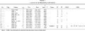
Table 1 shows the numbers of H, P1, and P2 groups for different group richness (number n of galaxy members). By applying the nonparametric Kolmogorov-Smirnov and sign statistical tests (e.g., Hoel 1971), we find no significant differences between the distributions. Thus, the three catalogs of groups are, on average, similar as far as the distribution of galaxy members in groups is concerned.
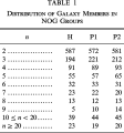 | Table 1 Distribution of Galaxy Members in NOG Groups |
Furthermore, we quantify the similarity between the catalogs of groups by counting the number of members of an H group that belong to a common P1 group. We first determine which members of each P1 group belong to the same H group. We calculate a largest group fraction (LGF) for each P1 group by dividing the number of members in the largest such subgroup by the total number of members in the P1 group (see Frederic 1995a for a similar definition of LGF). Figure 5 shows, as a function of group richness (number of members), the fraction of P1 groups of a given richness with LGFs of unity and in each quartile below. For example, there are 22 P1 groups with seven members. Of these, 48% have an LGF of 100%, 57% have an LGF of 75%, 91% have an LGF of at least 50%, and all of the n = 7 groups have LGFs greater than 25%. The H groups give a similar histogram, with somewhat greater values along the ordinate axis (see Fig. 6). The large fractions of groups having high LGF values confirm the similarity between the two catalogs of groups. If we repeat these calculations replacing P1 groups with P2 groups, we find slightly lower values along the ordinate axis in the plot corresponding to Figure 5 and an almost equal histogram in the plot corresponding to Figure 6. Thus, P1 groups are in slightly better agreement with H groups than P2 groups. If we compare P1 and P2 groups in the same way, we find a very good agreement, as expected (the values of LGF are almost always greater than 80% and are frequently greater than 90%).
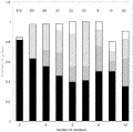
| Fig. 5 Histogram of the largest group fraction (LGF) as a function of the number of galaxy members in P1 groups. Solid black regions give the fraction of P1 groups with LGFs of unity, cross-hatched regions correspond to groups with LGF between 75% and 100%, single narrow-hatched regions correspond to LGFs between 50% and 75%, and no hatching represents groups with LGFs between 25% and 50%. The number at the top of each bar is the total number of P1 groups with the given number of members, n. The n = 10 bar includes all groups with 10 or more members. |
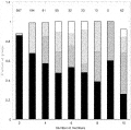
| Fig. 6 Histogram of the largest group fraction (LGF) as a function of the number of galaxy members in H groups. Hatching as in Fig. 5. |
Furthermore, we have calculated the LGF values separately for the nearby and distant NOG galaxies, dividing the sample at 3500 km s-1. In this way, we have verified that the agreement between the P1 and P2 groups gets slightly worse as we go to larger distances, as expected. On the other hand, there is no appreciable effect of this kind in the comparison between H and P1 (or P2) groups.
The ratio of the number of groups with at least three members to the number of nonmember (binary and field) galaxies is 0.12, 0.13, and 0.14 for the H, P1, and P2 groups, respectively. These values lie in the range of published values from other group catalogs, e.g., 0.09 for the SSRS1 groups (Maia et al. 1989), 0.10 for the LCRS groups (Tucker et al. 1997) and the PPS groups (Trasarti-Battistoni 1998), 0.11 for the PGC groups (Gourgoulhon et al. 1992; Fouqué et al. 1992), 0.12 for the SSRS2 groups (M. Ramella et al. 2000 in preparation), 0.13 for the CfA2 north (Ramella et al. 1997) and ESP groups (Ramella et al. 1999), 0.14 for the revised CfA1 groups (Nolthenius 1993), 0.17 for the NBG groups (Tully 1987), and 0.15 and 0.19 for the LEDA groups derived by Garcia (1993) using the P and H methods, respectively.
The ratio of members of groups with at least three members to the total number of galaxies is 0.44, 0.46, and 0.47 for the H, P1, and P2 groups, respectively, whereas published values are 0.35 for the SSRS1 (Maia et al. 1989), LCRS (Tucker et al. 1997), and PPS groups (Trasarti-Battistoni 1998), 0.40 for the SSRS2 groups (M. Ramella et al. 2000 in preparation), 0.41 for the ESP groups (Ramella et al. 1999), 0.42 for the PGC groups (Gourgoulhon et al. 1992; Fouqué et al. 1992), 0.45 for the CfA2 north groups (Ramella et al. 1997), 0.48 for the revised CfA1 groups (Nolthenius 1993), 0.51 for the NBG groups (Tully 1987), and 0.63 and 0.47 for the LEDA groups (Garcia 1993) derived by means of the P and H methods, respectively.
In general, our catalogs of groups are broadly consistent with the previous catalogs of groups selected in the same regions, and our values for the two above-mentioned ratios appear to be consistent with typical values reported in the literature.
As regards the H groups, our values are close to those of the PGC groups and are a little lower than those of the NBG groups (because we adopt a greater limiting luminosity density parameter to cut the hierarchy; see § 4.1). Compared to the LEDA groups identified with the H method, we find fewer groups, which is partially due to the fact that in many cases, Garcia (1993) neglected the reconstruction of high-velocity systems, which the algorithm tends to break into several systems with different average velocities (see § 4.1). Furthermore, compared to the LEDA groups identified with the P method, we basically find smaller groups with fewer members because, on average, we adopt lower values of czL (see § 4.2). In general, there is much less similarity between the two catalogs of LEDA groups than between our two catalogs.
A comparison of the distribution of the centers of the two samples of groups with that of galaxies shows qualitatively that groups trace the large-scale structure of the nearby universe.
The final catalogs of the members of the H, P1, and P2 groups are presented in Tables 2, 3, and 4, respectively. In these tables we give the NOG group number, the PGC and alternative names of the galaxy member, the 1950 right ascension and declination (in hours, minutes, seconds and degrees, arcminutes, and arcseconds, respectively), the velocity cz (in the Local Group frame), and its reference source (L = LEDA, O = other sources, e.g., NED, UZC, ORS, and PSCz), the corrected total blue magnitude, and its reference source. In the last column, "L" denotes the galaxies that have B magnitudes taken from LEDA and strictly constitute the NOG sample. We also include in the tables some additional galaxy members (omitted in the above-mentioned statistics), which are part of a small extension of the NOG containing 156 additional galaxies. These objects have rough estimates of B magnitudes (with B 14 mag) derived from diameters or from other recent sources (they are denoted by E or O, respectively).
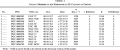 | Table 2 Galaxy Members of the Hierarchical (H) Catalog of Groups |
 | Table 3 Galaxy Members of the Percolation (P1) Catalog of Groups |
 | Table 4 Galaxy Members of the Percolation (P2) Catalog of Groups |
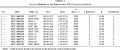
The final catalogs of H, P1, and P2 groups are presented in Tables 5, 6, and 7, respectively. In these tables we give the NOG group number, the name of the brightest galaxy of the group, the number of galaxy members, the median values of the 1950 right ascension and declination of the group members, the median value of recession velocity cz (in the Local Group frame), the common name of the system (when available), the cross-identifications between NOG groups, and the cross-identification between NOG groups and previous catalogs of groups. Of these we choose the all-sky catalogs of nearby groups published by Tully (1987; NBG) and Garcia (1993; LEDA) for a detailed comparison. Specifically, we consider Garcia's (1993) final catalog of groups, defined by her as the one that includes only systems common to the two original catalogs that she constructed by means of the H and P methods. Cross-identifications are tabulated only when there are at least three galaxies in common between our groups (with at least three members) and groups of previous catalogs, and two galaxies in common between pairs. Some additional galaxy members, which are part of a small extension of the NOG (see above), are included in the Tables. The statistics on group catalogs as mentioned above can be obtained by omitting these additional galaxies.
 | Table 5 Catalog of the Hierarchical (H) Groups |
 | Table 6 Catalog of the Percolation (P1) Groups |
 | Table 7 Catalog of the Percolation (P2) Groups |
In Table 5 we denote by an asterisk the 17 systems that are split by the H algorithm along the line of sight and then reconstructed by us with the aid of the results of the P1 method. Moreover, in Table 5 we denote by a plus sign in the "flag" column the 11 systems that are constructed with the aid of membership assignments provided directly in the literature for the Virgo region and for four very nearby groups (see § 4.1). As explained at the end of § 4.2, the P1 and P2 systems are by definition taken to be equal to those identified with the H method in the Virgo region and in the very nearby region (cz < 500 km s-1). These systems are also denoted by a plus sign in the "flag" column in Tables 6 and 7.
Tables 27 can be found in their entirety in the electronic version of this article.
6. CONCLUSIONS
In this paper we describe the NOG sample, a distance-limited (cz < 6000 km s-1) and magnitude-limited (B 14 mag) sample of 7076 optically selected galaxies that covers 2/3 of the sky (|b| > 20) and has a good completeness in redshift (97%).
We select the NOG on the basis of homogenized corrected blue magnitudes in order to minimize systematic effects in galaxy sampling due to the use of different magnitude systems in different areas of the sky and to Galactic and internal extinction. In this sense, the NOG, which is meant to be the first step toward the construction of a statistically well-controlled optical galaxy sample with homogenized photometric data covering most of the celestial sphere, is in principle designed to offer a largely unbiased view of the galaxy distribution.
We identify galaxy systems in the NOG by means of both hierarchical and percolation friends-of-friends methods. After an extensive search in the space of relevant parameters with the guide of available numerical simulations, we choose optimal sets of parameters that allow us to obtain reliable and homogeneous catalogs of loose groups. Remarkably, these catalogs turn out to be substantially consistent as far as the distribution of members in groups is concerned. Containing about 500 systems (with at least three members), they are among the largest catalogs of groups currently available. Although they are drawn from a galaxy sample limited to bright magnitudes, they are useful for studying the statistical properties of loose groups, since their physical properties were found to be stable, on average, against the inclusion of fainter galaxy members (Ramella et al. 1995a, 1995b; Ramella, Focardi, & Geller 1996). In particular, being extracted from the same galaxy sample, the catalogs allow one to investigate variations in group properties (e.g., velocity dispersion, virial mass and radius) strictly related to differences in the algorithm adopted. These differences indicate to what extent our knowledge of the location and properties of groups in the nearby universe is inaccurate. Previous comparisons between catalogs of groups identified with the H and P algorithms (Pisani et al. 1992) were based on catalogs extracted from different galaxy samples.
Most of the NOG galaxies (60%) are found to be members of galaxy pairs (580 pairs, comprising 15% of the galaxies) or groups with at least three members (500 groups, comprising 45% of the galaxies). About 40% of the galaxies are left ungrouped (field galaxies).
Although limited to a depth of 6000 km s-1, the NOG covers interesting regions of prominent overdensities (in mass and galaxies) of the nearby universe, such as the "Great Attractor" region and the Perseus-Pisces supercluster. Compared to previous all-sky optical and IRAS galaxy samples, the NOG provides a denser sampling of the galaxy density field in the nearby universe. In addition, as expected, the NOG delineates overdensity regions with a greater density contrast than IRAS galaxy samples do.
Given its high density sampling and large sky coverage, the NOG sample is well suited to mapping the cosmography of the nearby universe beyond the Local Supercluster and for allowing a comparison of the density field as traced by optical galaxies with that described by IRAS galaxies (addressing questions concerning the amount of relative biasing in the galaxy distribution and its possible dependence on scale).
By virtue of the identification of NOG groups, the NOG is also well suited to deriving galaxy density parameters on small scales to be used in observational investigations of environmental effects on galaxy properties. Environmental studies in which the local galaxy density is decoupled from membership in galaxy systems go beyond the conventional comparison between the properties of cluster and field galaxies and thus can better constrain the physical processes responsible for the formation and evolution of galaxies. Much of the observed evolution of the properties and populations of galaxies (e.g., Ellis 1997) that has occurred during recent epochs (z < 1) can be ascribed to interaction of galaxies and their local environment.
In a subsequent paper (see Marinoni et al. 2000 for preliminary results), the NOG groups will be used to remove nonlinearities in the peculiar-velocity field (e.g., the velocity dispersion of group members) on small scales. To correct the redshift distances of field galaxies and groups on large scales, we will apply models of the peculiar velocity field, following the approach described in Paper I. We will use the locations of individual galaxies and groups calculated in real-distance space (i.e., for distances predicted by different velocity field models) to calculate the selection function of the NOG sample (see Paper II) and to reconstruct the galaxy density field. Local galaxy density parameters to be used in studies of environmental effects on nearby galaxies will be provided.
We are indebted to B. Santiago (together with the ORS team) and to W. Saunders (together with the PSCz team) who provided us with data in advance of publication. We wish to thank S. Borgani, D. Fadda, R. Giovanelli, M. Girardi, M. Hudson, F. Mardirossian, M. Mezzetti, P. Monaco, and M. Ramella for interesting conversations. C. M. and L. C. are grateful to SISSA for its kind hospitality. This research has made use of the Lyon-Meudon Extragalactic Database (LEDA), supplied by the LEDA team at the CRAL-Observatoire de Lyon (France), and the NASA/IPAC Extragalactic Database (NED), which is operated by the Jet Propulsion Laboratory, California Institute of Technology, under contract to the National Aeronautics and Space Administration. This work has been partially supported by the Italian Ministry of University, Scientific and Technological Research (MURST) and by the Italian Space Agency (ASI).
REFERENCES
- Arce, H. G., & Goodman, A. A. 1999, ApJ, 512, L135 First citation in article | Full Text | NASA ADS
- Baker, J. E., Davis, M., Strauss, M. A., Lahav, O., & Santiago, B. X. 1998, ApJ, 508, 6 First citation in article | Full Text | NASA ADS
- Binggeli, B., Popescu, C. C., & Tammann, G. A. 1993, A&AS, 98, 275 First citation in article | NASA ADS
- Binggeli, B., Sandage, A., & Tammann G. A. 1985, AJ, 90, 1681 First citation in article | NASA ADS
- Binggeli, B., Tammann, G. A., & Sandage, A. 1987, AJ, 94, 251 First citation in article | NASA ADS
- Branchini, E., et al. 1999, MNRAS, 308, 1 First citation in article | NASA ADS
- Burstein, D., & Heiles, C. 1978, ApJ, 225, 40 First citation in article | NASA ADS
- . 1982, AJ, 87, 1165 First citation in article | NASA ADS
- Burstein, D., et al. 1987, ApJS, 64, 601 First citation in article | NASA ADS
- Côté, S., Freeman, K. C., Carignan, C., & Quinn, P. J. 1997, AJ, 114, 1313 First citation in article | NASA ADS
- da Costa, L. N., et al. 1988, ApJ, 327, 544 First citation in article | NASA ADS
- Davis, M., Huchra, J., Latham, D. W., & Tonry, J. 1982, ApJ, 253, 423 First citation in article | NASA ADS
- de Lapparent, V., Geller, M. J., & Huchra, J. P. 1989, ApJ, 343, 1 First citation in article | NASA ADS
- de Vaucouleurs, G., et al. 1991, Third Reference Catalogue of Bright Galaxies (New York: Springer) (RC3) First citation in article
- Diaferio, A., Kauffmann, G., Colberg, J. M., & White, S. D. M. 1999, MNRAS, 307, 537 First citation in article | NASA ADS
- Ellis, R. S. 1997, ARA&A, 35, 389 First citation in article | NASA ADS
- Epchtein, N., et al. 1999, A&A, 349, 236 First citation in article | NASA ADS
- Escalera, E., & MacGillivray, H. T. 1995, A&A, 298, 1 First citation in article | NASA ADS
- Fairall, A. 1998, Large-Scale Structures in the Universe (Chichester: John Wiley & Sons) First citation in article
- Falco, E. E., et al. 1999, PASP, 111, 438 First citation in article | Full Text | NASA ADS
- Federspiel, M., Tammann, G. A., & Sandage, A. 1998, ApJ, 495, 115 First citation in article | Full Text | NASA ADS
- Fisher, K. B., Davis, M., Strauss, M. A., Yahil, A., & Huchra, J. P. 1995, ApJS, 100, 69 First citation in article | NASA ADS
- Focardi, P., Marano, B., & Vettolani, G. 1986, A&A, 161, 217 First citation in article | NASA ADS
- Fouqué, P., Gourgoulhon, E., Chamaraux, P., & Paturel, G. 1992, A&AS, 93, 211 First citation in article | NASA ADS
- Frederic, J. J. 1995a, ApJS, 97, 259 First citation in article | NASA ADS
- . 1995b, ApJS, 97, 275 First citation in article | NASA ADS
- Garcia, A. M. 1993, A&AS, 100, 47 First citation in article | NASA ADS
- Gavazzi, G., Boselli, A., Scodeggio, M., Pierini, D., & Belsole, E. 1999, MNRAS, 304, 595 First citation in article | NASA ADS
- Geller, M., & Huchra, J. P. 1983, ApJS, 52, 61 First citation in article | NASA ADS
- Giovanelli, R., et al. 1995, AJ, 110, 1059 First citation in article | NASA ADS
- . 1997, AJ, 113, 22 First citation in article | NASA ADS
- Girardi, M., & Giuricin, G. 2000, ApJ, 540, 45 First citation in article | Full Text | NASA ADS
- Giudice, G. 1999, in ASP Conf. Ser. 176,
Observational Cosmology: The Development of Galaxy Systems, ed. G.
Giuricin, M. Mezzetti, & P. Salucci (San Francisco: ASP), 136 First citation in article
- Giuricin, G., Limboz Tektunali, F., Monaco, P., Mardirossian, F., & Mezzetti, M. 1995, ApJ, 450, 41 First citation in article | NASA ADS
- Giuricin, G., Mardirossian, F., Mezzetti, M., & Monaco, P. 1993, ApJ, 407, 22 First citation in article | NASA ADS
- Giuricin, G., Monaco, P., Mardirossian, F., & Mezzetti, M. 1994, ApJ, 425, 450 First citation in article | NASA ADS
- Gourgoulhon, E., Chamaraux, P., & Fouqué, P. 1992, A&A, 255, 69 First citation in article | NASA ADS
- Hermit, S., et al. 1996, MNRAS, 283, 709 First citation in article | NASA ADS
- Hoel, P. G. 1971, Introduction to Mathematical Statistics (New York: Wiley) First citation in article
- Huchra, J. P., & Geller, M. 1982, ApJ, 257, 423 First citation in article | NASA ADS
- Huchra, J. P., 2000, in ASP Conf. Ser. 201, Cosmic
Flows Workshop, ed. S. Courteau, M. A. Strauss & J. Willick (San
Francisco: ASP), 96 First citation in article
- Hudson, M. J. 1993a, MNRAS, 265, 43 First citation in article | NASA ADS
- . 1993b, MNRAS, 265, 72 First citation in article | NASA ADS
- . 1994a, MNRAS, 266, 468 First citation in article | NASA ADS
- . 1994b, MNRAS, 266, 475 First citation in article | NASA ADS
- . 1999, PASP, 111, 57 First citation in article | Full Text | NASA ADS
- Joint IRAS Science Working Group. 1988, IRAS Point Source Catalog, Version 2 (Washington: GPO) First citation in article
- Lauberts, A. 1982, The ESO-Uppsala Survey of the ESO (B) Atlas (München: ESO) First citation in article
- Lauberts, A., & Valentijn, E. 1989, The Surface Photometry Catalogue of the ESO-Uppsala Galaxies (München: ESO) First citation in article
- Lu, N. Y., & Freudling, W. 1995, ApJ, 449, 527 First citation in article | NASA ADS
- Maia, M. A. G., da Costa, L. N., & Latham, D. W. 1989, ApJS, 69, 809 First citation in article | NASA ADS
- Marinoni, C., Giuricin, G., Ceriani, L., &
Pisani A. 2000, in ASP Conf. Ser. 201, Cosmic Flows Workshop, ed. S.
Courteau, M. A. Strauss & J. Willick (San Francisco: ASP), 314 First citation in article
- Marinoni, C., Monaco, P., Giuricin, G., & Costantini, B. 1998, ApJ, 505, 484 (Paper I) First citation in article | Full Text | NASA ADS
- . 1999, ApJ, 521, 50 (Paper II) First citation in article | Full Text | NASA ADS
- Mateo, M. 1998, ARA&A, 36, 435 First citation in article | NASA ADS
- Materne, J. 1978, A&A, 63, 401 First citation in article | NASA ADS
- Mitra, S. 1989, AJ, 98, 1175 First citation in article | NASA ADS
- Monaco, P., Giuricin, G., Mardirossian, F., & Mezzetti, M. 1994, ApJ, 436, 576 First citation in article | NASA ADS
- Moore, B., Frenk, C. S., & White S. D. M. 1993, MNRAS, 261, 827 First citation in article | NASA ADS
- Nakanishi, K., et al. 1997, ApJS, 112, 245 First citation in article | Full Text | NASA ADS
- Nilson, P. 1973, Uppsala General Catalogue of Galaxies (Uppsala: Uppsala Astron. Obs. Ann. 6) (UGC) First citation in article
- Nolthenius, R. 1993, ApJS, 85, 1 First citation in article | NASA ADS
- Nolthenius, R., Klypin, A. A., & Primack, J. R. 1994, ApJ, 422, L45 First citation in article | NASA ADS
- . 1997, ApJ, 480, 43 First citation in article | Full Text | NASA ADS
- Nolthenius, R., & White, S. D. M. 1987, MNRAS, 225, 505 First citation in article | NASA ADS
- Paturel, G., et al. 1997, A&AS, 124, 109 First citation in article | NASA ADS
- Pellegrini, P. S., et al. 1990, AJ, 99, 751 First citation in article | NASA ADS
- Pisani, A. 1996, MNRAS, 278, 697 First citation in article | NASA ADS
- Pisani, A., Giuricin, G., Mardirossian, F., & Mezzetti, M. 1992, ApJ, 389, 68 First citation in article | NASA ADS
- Ramella, M., Focardi, P., & Geller, M. J. 1996, A&A, 312, 745 First citation in article | NASA ADS
- Ramella, M., Geller, M. J., & Huchra, J. P. 1989, ApJ, 344, 57 First citation in article | NASA ADS
- Ramella, M., Geller, M. J., Huchra, J. P., & Thorstensen, J. R. 1995a, AJ, 109, 1458 First citation in article | NASA ADS
- . 1995b, AJ, 109, 1469 First citation in article | NASA ADS
- Ramella, M., Pisani, A., & Geller, M. J. 1997, AJ, 113, 483 First citation in article | NASA ADS
- Ramella, M., et al. 1999, A&A, 342, 1 First citation in article | NASA ADS
- Sandage, A., & Tammann, G. A. 1981, Revised Shapley-Ames Catalog (Washington: Carnegie Inst.) (RSA) First citation in article
- Santiago, B. X., et al. 1995, ApJ, 446, 457 First citation in article | NASA ADS
- . 1996, ApJ, 461, 38 First citation in article | NASA ADS
- Saunders, W., et al. 1991, Nature, 349, 32 First citation in article | NASA ADS
- . 2000a, MNRAS, 317, 55 First citation in article | NASA ADS
- . 2000b, in ASP Conf. Ser. 201, Cosmic Flows Workshop, ed. S. Courteau, M. A. Strauss & J. Willick (San Francisco: ASP), 223 First citation in article
- Schechter, P. 1976, ApJ, 203, 297 First citation in article | NASA ADS
- Schlegel, D. J., Finkbeiner, D. P., & Davis, M. 1998, ApJ, 500, 525 First citation in article | Full Text | NASA ADS
- Schmoldt, I. M., et al. 1999, AJ, 118, 1146 First citation in article | Full Text | NASA ADS
- Strauss, M. A. 1999, in Formation of Structure in
the Universe, ed. A. Dekel & J. Ostriker (Cambridge: Cambridge
Univ. Press), 172 First citation in article
- Strauss, M. A., Davis, M., Yahil, A., Fisher, K., & Tonry, J. P. 1992, ApJ, 385, 421 First citation in article | NASA ADS
- Takata, T., Yamada, T., & Sait, M. 1996, ApJ, 457, 693 First citation in article | NASA ADS
- Trasarti-Battistoni, R. 1998, A&AS, 130, 341 First citation in article | NASA ADS
- Tucker, D. L. et al. 1997, preprint (astro-ph/9711176) First citation in article
- Tully, R. B. 1980, ApJ, 237, 390 First citation in article | NASA ADS
- . 1987, ApJ, 321, 280 First citation in article | NASA ADS
- . 1988, Nearby Galaxies Catalog (Cambridge: Cambridge Univ. Press) (NBG) First citation in article
- Tully, R. B., & Fisher, J. R. 1987, Nearby Galaxies Atlas (Cambridge: Cambridge Univ. Press) First citation in article
- Turner, E. L. 1979, ApJ, 231, 645 First citation in article | NASA ADS
- van Driel, W., Kraan-Korteweg, R. C., Binggeli, B., & Huchtmeier, W. K. 1998, A&AS, 127, 397 First citation in article | NASA ADS
- Vennik, J. 1984, Tartu Astr. Obs. Publ., 73, 1 First citation in article
- Vorontsov-Velyaminov, B. A., Archipova, V. P., & Krasnogorskaja, A. A. 19621974, Morphological Catalogue of Galaxies, Vols. 15 (Moscow: Moscow State Univ.) (MCG) First citation in article
- Yahil, A., Sandage, A., & Tammann, G. A. 1980, ApJ, 242, 448 First citation in article | NASA ADS
- Yahil, A., Tammann, G. A., & Sandage, A. 1977, ApJ, 217, 903 First citation in article | NASA ADS
- Yasuda, N., Fukugita, M., & Okamura, S. 1997, ApJS, 108, 417 First citation in article | Full Text | NASA ADS
- Wakamatsu, K., et al. 1994, in ASP Conf. Ser. 67,
Unveiling Large-Scale Structure behind the Milky Way, ed. C. Balkowski
& R. C. Krann-Korteweg (San Francisco: ASP), 131 First citation in article
- Webster, M., Lahav, O., & Fisher, K. 1997, MNRAS, 287, 425 First citation in article | NASA ADS
- Wegner, G., Haynes, M. P., & Giovanelli, R. 1993, AJ, 105, 1251 First citation in article | NASA ADS
- Zwicky, F., et al. 19611968. Catalog of Galaxies and Clusters of Galaxies, Vols. 16 (Pasadena: California Inst. Technology) (CGCC) First citation in article